


This function, applied to the high level and low level data points, yields new
threshold vs. value combinations.
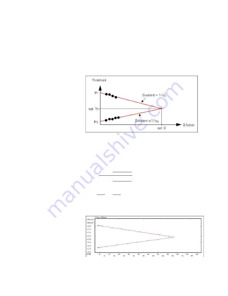
In the area of low BER (typically below 10
-4
), these new data pairs should fit to two
straight lines, although a couple of assumptions and approximations have been
made.
To determine the gradient and offset of these lines, a linear regression is performed.
This is illustrated in the figure below.
A straight line can be expressed as:
Y = A + BX
where Y is the inverse error function of BER, and X is D, the decision threshold.
The following calculations are performed for the high and low level data:
S
XY
- (S
X
)(S
Y
)
n
S
X
2
-
(S
X
)
2
n
B =
S
Y
n
A =
- B
S
X
n
where n is the number of respective data points.
The results of the linear regression are displayed in the
QBER vs. Threshold
graph.
6
Advanced Analysis
284
Agilent J-BERT N4903B High-Performance Serial BERT
Summary of Contents for J-BERT N4903B
Page 1: ...S Agilent J BERT N4903B High Performance Serial BERT User Guide s Agilent Technologies ...
Page 10: ...10 Agilent J BERT N4903B High Performance Serial BERT ...
Page 36: ...1 Planning the Test 36 Agilent J BERT N4903B High Performance Serial BERT ...
Page 60: ...2 Setting up External Instrument s 60 Agilent J BERT N4903B High Performance Serial BERT ...
Page 120: ...3 Setting up Patterns 120 Agilent J BERT N4903B High Performance Serial BERT ...
Page 360: ...6 Advanced Analysis 360 Agilent J BERT N4903B High Performance Serial BERT ...
Page 468: ...8 Jitter Tolerance Tests 468 Agilent J BERT N4903B High Performance Serial BERT ...
Page 524: ...9 Solving Problems 524 Agilent J BERT N4903B High Performance Serial BERT ...
Page 566: ...10 Customizing the Instrument 566 Agilent J BERT N4903B High Performance Serial BERT ...