LeCroy SDA, Руководство оператора

Страница: 387 / 397

SDA Operator’s Manual
Interpretation of TIE Histogram – the Distribution of Edge Transition Times vs. Ideal (Expected)
Transition Times
For the purposes of this discussion (in connection with jitter measurement
10
) the entire subject
surrounds the matter of interpreting the observed distribution of timing errors. This observed
distribution is the histogram of Time Interval Error (TIE) values, obtained through analysis of
either clock or NRZ data waveforms acquired by a digital recording instrument (such as a digital
oscilloscope).
Relationship between Histograms and PDF
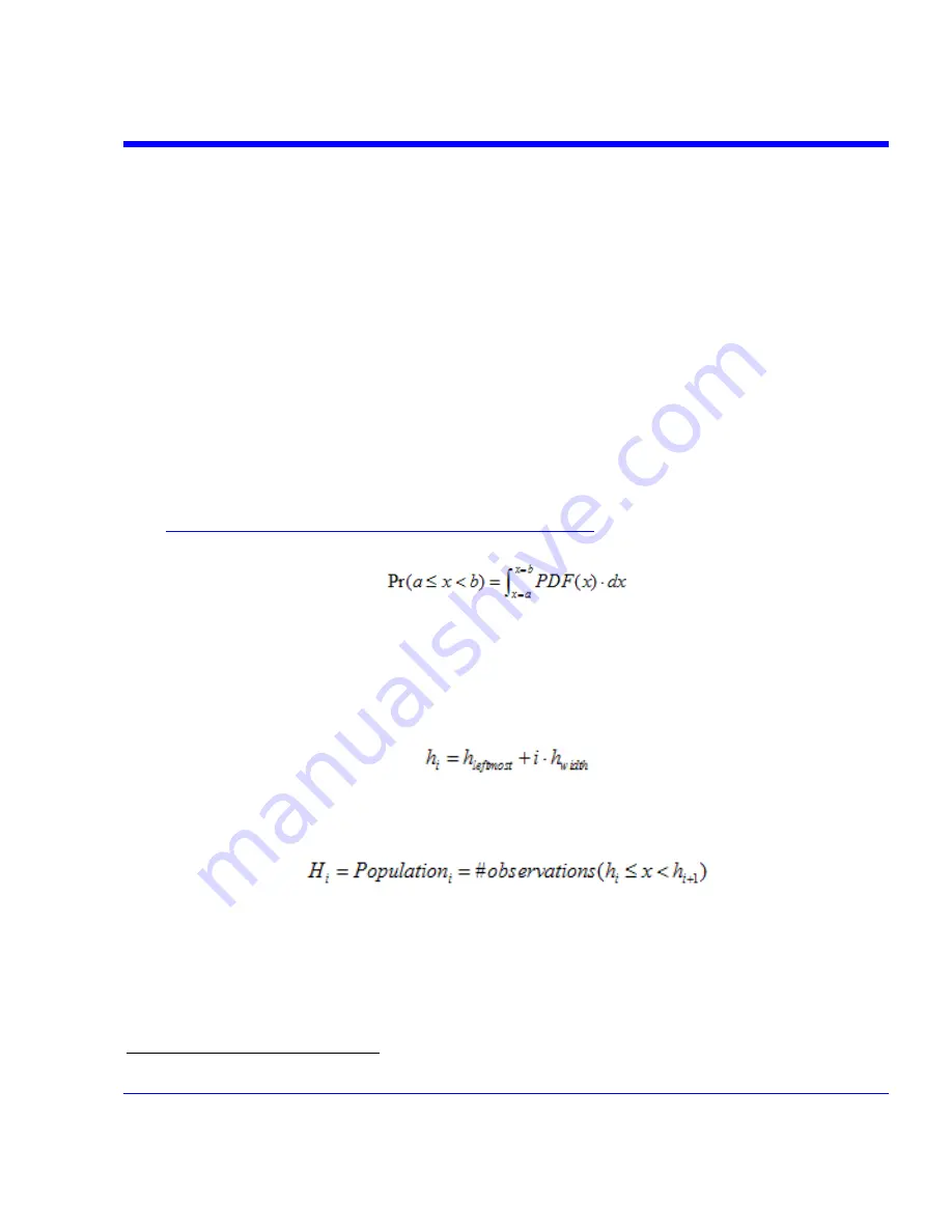
A histogram is nothing more than a form of data representation that expresses the frequency of
occurrence of measurement values sorted or “binned” into adjacent, equal width contiguous
intervals (or bins). When the timing errors (TIE) are collected as a histogram, the histogram
serves as an approximation to the Probability Density Function (PDF) of this statistically based
phenomenon (jitter). The PDF is (in theory) a smooth function determined by the underlying
physics of the measured phenomenon (and of course what we actually observe includes the
physics of the instrumentation as well).
The PDF is a continuous function, and reflects integrals of the probability
(see
http://en.wikipedia.org/wiki/Probability_density_function ) over each interval of measurem
value, x .
ent
That is to say, the density of probability as a function of the measured quantity when integrated
over a given region gives the probability that any measurement value will be within that region.
The process of forming a histogram is based upon a pre-specified set of bin boundaries (meeting
the above conditions of contiguity and equal width). A further constraint, which is usually
unspoken, is that the histogram range must cover all possible observation values if it is to be
useful.
The set of observations (of measured quantity
x ) are “binned” or counted for each range of
histogram bin. The resulting histogram is a collection of populations (or counts) for each bin
region.
Now a measurement histogram (like the one we will analyze to estimate jitter) represents a single
experiment, with some number of trials or individual TIE measured values. It is only an
approximation of the PDF insofar as the true PDF plays its probabilistic role and so is reflected in
the resulting observations.
SDA-OM-E Rev H
387
10
The “normalized Q-scale” method can be applied to other statistical studies and measurements; in particular, for
examining the nature of vertical noise distributions.