As the bathtub borders are not uniform (both have two edges), the linear
derivative (the jitter) will show two peaks:
If you switch to linear scale and enable the marker, you can see its bell
shape.
You can measure the random jitter distribution of each peak as well as
the distance between the peaks, which means the deterministic jitter.
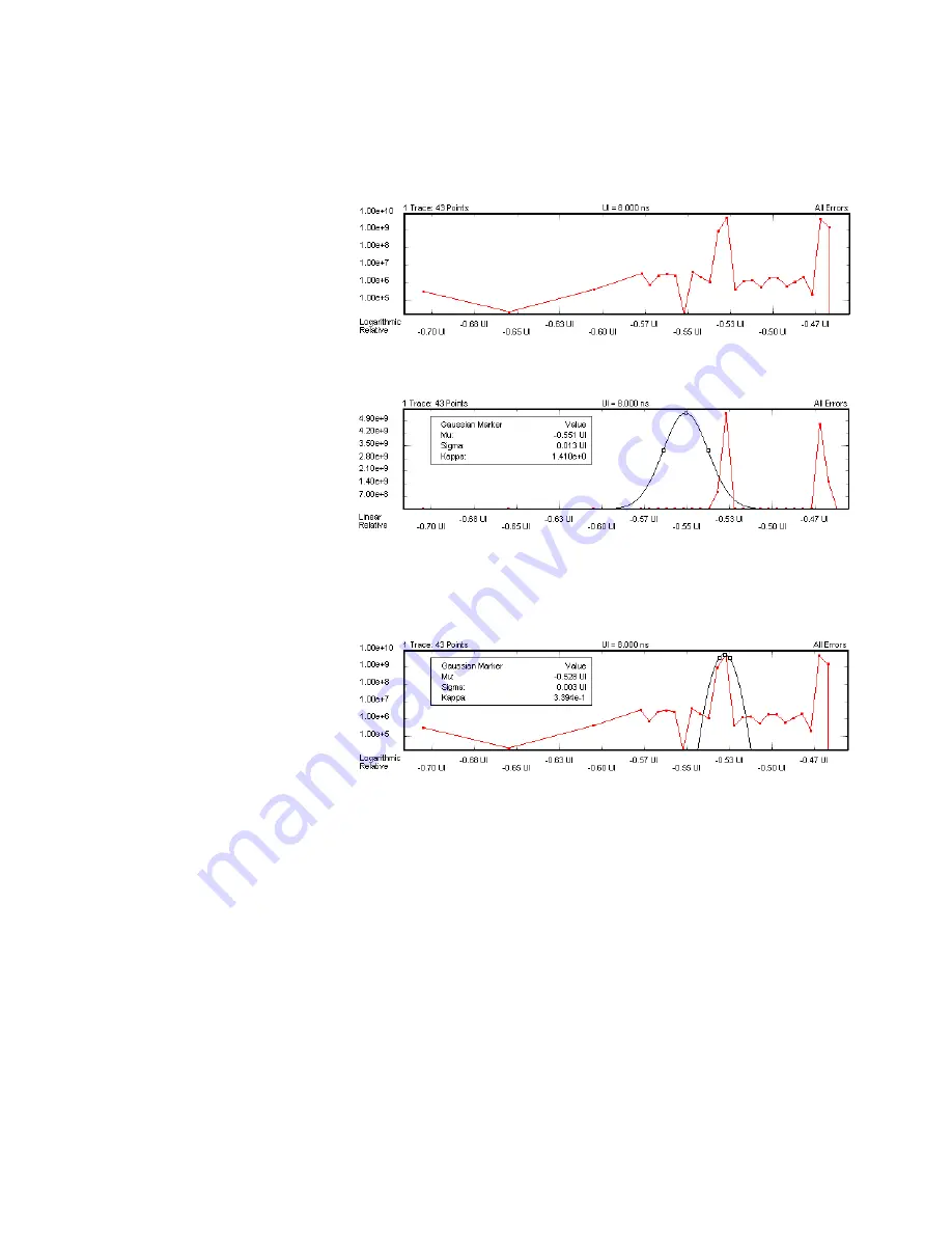
You can also use the marker with logarithmic scale. In this case, it
appears as a parabolic curve:
A Gaussian marker is used when the dBER vs. Threshold Graph is
displayed. This graph shows the relationship between the decision
threshold and the absolute values of the derivative of the bit error rate
(dBER/dTh). A linear scale reveals the distribution more clearly than a
logarithmic scale (see
“dBER vs. Threshold Graph” on page 207
In the example below,
μ
(Mu) and
σ
(Sigma) will be the same as the Level
and Standard Deviation results calculated by the measurement.
5
Advanced Analysis
172
Agilent J-BERT N4903 High-Performance Serial BERT
Output Levels measurement
Summary of Contents for J-BERT N4903
Page 1: ...S Agilent J BERT N4903 High Performance Serial BERT User Guide s Agilent Technologies...
Page 68: ...2 Setting up Patterns 68 Agilent J BERT N4903 High Performance Serial BERT...
Page 158: ...4 Setting up the Error Detector 158 Agilent J BERT N4903 High Performance Serial BERT...
Page 314: ...6 Evaluating Results 314 Agilent J BERT N4903 High Performance Serial BERT...
Page 374: ...7 Jitter Tolerance Tests 374 Agilent J BERT N4903 High Performance Serial BERT...
Page 394: ...8 Solving Problems 394 Agilent J BERT N4903 High Performance Serial BERT...
Page 434: ...Index 434 Agilent J BERT N4903 High Performance Serial BERT...