HP 50G, User Manual

Page: 468 / 887

Page 14-8
The resulting matrix has elements a
11
=
∂
2
φ
/
∂
X
2
= 6., a
22
=
∂
2
φ
/
∂
X
2
= -2.,
and a
12
= a
21
=
∂
2
φ
/
∂
X
∂
Y = 0. The discriminant, for this critical point s2(1,0)
is
Δ
= (
∂
2
f/
∂
x
2
)
⋅
(
∂
2
f/
∂
y
2
)-[
∂
2
f/
∂
x
∂
y]
2
= (6.)(-2.) = -12.0 < 0, indicating a
saddle point.
Multiple integrals
A physical interpretation of an ordinary integral, , is the area under
the curve y = f(x) and abscissas x = a and x = b. The generalization to three
dimensions of an ordinary integral is a double integral of a function f(x,y) over
a region R on the x-y plane representing the volume of the solid body contained
under the surface f(x,y) above the region R. The region R can be described as
R = {a<x<b, f(x)<y<g(x)} or as R = {c<y<d, r(y)<x<s(y)}. Thus, the double
integral can be written as
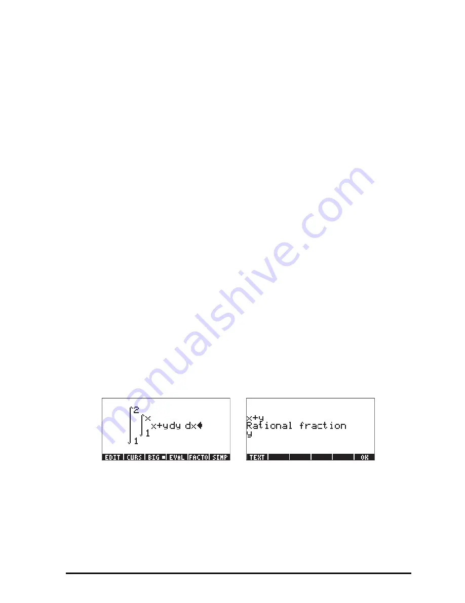
Calculating a double integral in the calculator is straightforward. A double
integral can be built in the Equation Writer (see example in Chapter 2). An
example follows. This double integral is calculated directly in the Equation
Writer by selecting the entire expression and using function
@EVAL
. The result is
3/2. Step-by-step output is possible by setting the Step/Step option in the CAS
MODES screen.
∫
b
a
dx x f
) (
∫ ∫ ∫ ∫ ∫∫
= =
d
c
y s
y r
b
a
x g
x f
R
dydx y x dydx y x dA y x
) (
) (
) (
) (
) , ( ) , ( ) , (
φ φ φ