


Setting
up Compax3
C3I20T11 / C3I32T11
196
192-120103 N13 C3I20T11 / C3I32T11 December 2010
The cascade control offers the following advantages:
Disturbances occurring within the control path, can be compensated in the
subordinate control loop. Therefore they must not pass through the entire control
path and are thus compensated earlier.
The delay times within the path can be reduced for the superposed controller.
The limitation of the intermediate variables can be made by the control variable
limitation of the superposed controller rather easily .
The effects of the non-linearity for the superposed controllers can be reduced by
the subordinate control loops.
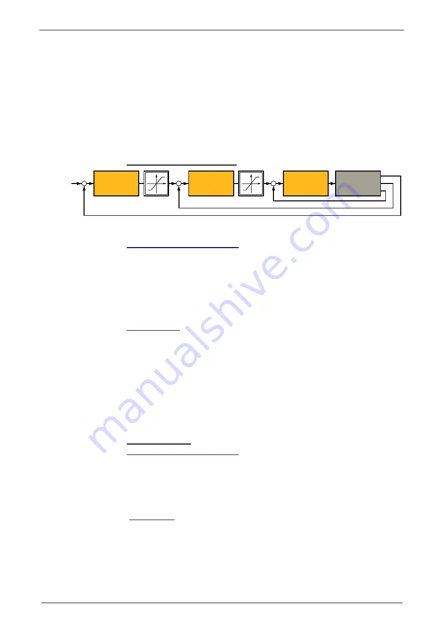
In the Compax3 servo drive, a triple cascade control is implemented with the
following controllers - position controller, velocity controller and current controller.
Cascade structure of Compax3
Current Controller
Stromregelung
Motor
Speed Controller
Drehzahlregelung
Position Controller
Positionsregler
Xw
X
n
i
Rigidity
In this chapter you can read about:
Static stiffness ............................................................................................................... 196
Dynamic stiffness .......................................................................................................... 196
Correlation between the terms introduced...................................................................... 198
The stiffness of a drive represents an important characteristic. The faster the
disturbance variable can be compensated in the velocity control path and the
smaller the oscillation caused, the higher the stiffness of the drive. With regard to
stiffness, we distinguish static and dynamic stiffness.
Static stiffness
The static stiffness of a direct drive is comparable with the spring rate D of a
mechanical spring, and indicates the excursion of the spring in the event of a
constant interference force. It is the ratio between the constant force FDmax of the
motor and a position difference. Due to the I term in the velocity controller, the
static stiffness is therefore infinitely high in theory, as the I term is integrated until
the control difference vanishes. In a digital control the static stiffness is above all
limited by the finite resolution of the position signal (the error must be at least one
quantization step, so that it can be detected by the reading system) and by
numerical resolution. Additional effects are for instance mechanical stiffness of the
mechanic components in the control path (e.g. load connection, guiding system) as
well as measurement errors of the measurement system.
Dynamic stiffness
In this chapter you can read about:
Traditional generation of a disturbance torque/force jerk ................................................ 197
Electronic simulation of a disturbance torque jerk with the disturbance current jerk........ 197
Disturbance jerk response ............................................................................................. 197
The dynamic stiffness is described by the ratio between the change in load torque
or in load force and the resulting position deviation (following error):
x
M
L
∆
∆
−
The higher this ratio (=dynamic stiffness), the higher the necessary change is load
torque in order to generate a defined following error.
The dynamic stiffness can be acquired from the disturbance jerk response.


