


98
PL12EN-1300 2008-03
en04d141.fm, 11.03.2008
Statistics
4
4.1.2
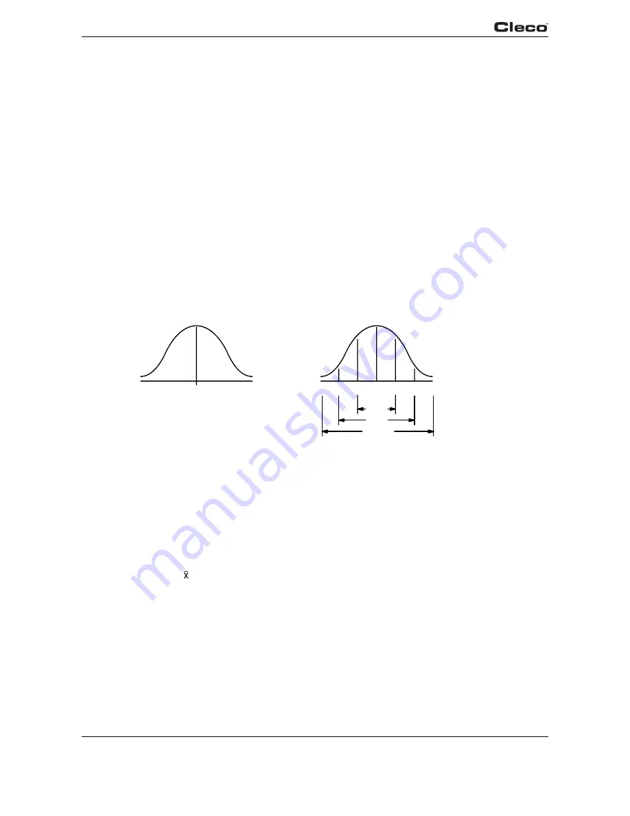
The Normal Curve
Most processes in statistical control have a fixed pattern of variation. The mathematical curve
that describes this pattern is known as the normal curve (see graph 4-2a). The normal curve is
symmetrical about the average. It is high in the middle and becomes smaller as the distance from
the average increases. Since the shape resembles a bell, it is sometimes referred to as a bell
curve.
The normal curve is defined by two conditions - the average of all items produced, and the
amount of variation from the average. We can think of these as the center and width of the bell,
respectively. The center is the arithmetic average of all items produced. The width is expressed
in terms of the standard deviation which is a statistical calculation for the amount of variation
from the average. The standard deviation, represented by the Greek letter sigma (
σ
), holds a
fixed relationship to the normal curve, as follows (see graph 4-2b):
• 68% of all items produced will be 1
σ
of the average (two sigma spread).
• 95% will be 2
σ
of the average (four sigma spread).
• 99.7% will be 3
σ
of the average (six sigma spread).
These two characteristics - the average and the standard deviation - provide the foundation for
statistical process control. By taking sample measurements during production, we can predict the
average value and the amount of variation for all items produced.
68%
95%
99.7%
1
σ
1
σ
2
σ
2
σ
3
σ
3
σ
Avg.
Avg.
Fig. 4-2: a) The Normal Curve Fig. 4-2: b) Areas Under The Normal Curve
4.1.3
The Procedure
The procedure for establishing a statistical process control program consists of three phases.
The first is to obtain statistical control - a state of random and stable variation. The second is to
establish process capability. A state of statistical control in itself does not assure that the process
is capable of meeting the specification. The limits of variation must be equal to or less than the
total specification tolerance. The third is to monitor the process throughout production using the
control chart, to detect and correct conditions that upset the stable pattern of variation.
Use of the -R Control Chart includes the following steps:
1.
Select the Characteristic
Since a separate chart is required for each characteristic, practical considerations limit use to
selected requirements. A good candidate is a characteristic that is important to the function of the
item. Others include those that are causing a high cost loss because of scrap or rework, and
those that require evaluation by destructive testing.