52
⑶
⑶
⑶
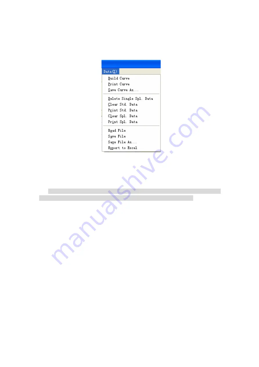
⑶ Save Curve As.
Save Curve As.
Save Curve As.
Save Curve As. Save
and rename the current curve.
⑷
⑷
⑷
⑷
Delete Single Spl. Data. Delete the data of a single sample from the sample column.
⑸
⑸
⑸
⑸
Clear Std. Data . Clear the data from the standard sample column.
⑹
⑹
⑹
⑹
Print Std. Data. Print the data of standard samples.
Fig. 2-18 Data Processing Sub-menu
⑺
⑺
⑺
⑺
Clear Spl. Data. Clear the data from the sample column.
⑻
⑻
⑻
⑻
Print Spl. Data. Print the data in the sample column.
⑼
⑼
⑼
⑼
Read File. Load the previously saved quantitation files from the hard disk.
Note: This function is often used to create a working curve by employing the previous data of
standard solutions so as to make a direct measurement for samples of the same kind.
①
After clicking “Build Curve” in “Data Processing” menu, you may see the working curve,
the equation and the correlation coefficient immediately.
②
After closing the window, place the sample into the light path and click “Measure Spl.”.
The concentration of the sample will be displayed on the screen.
⑽
⑽
⑽
⑽
Save File. Save the data in the quantitation files onto the hard disk. After clicking this item,
a dialog box will appear. Enter a name of the file and click “Save”.
⑾
⑾
⑾
⑾
Save File As. Save the data in the quantitation files onto the hard disk. Rename the new file
and click “Save”.
⑿
⑿
⑿
⑿
Send to Excel. The data in the quantitation files can be sent to Excel.
INSTRUCTION MANUAL FOR SPECTRO 96 FLUOROSPECTROPHOTOMETER


