


Chapter 12: Statistics
179
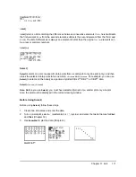
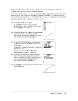
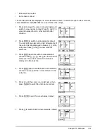
Since the scatter plot of time-versus-length data appears to be approximately linear, fit a line to the
data.
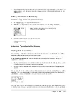
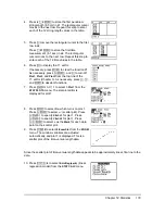
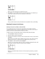
4. Press
6
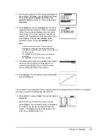
Ë
5
Í
to store the first pendulum
string length (6.5 cm) in
L1
. The rectangular cursor
moves to the next row. Repeat this step to enter
each of the 12 string length values in the table.
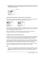
5. Press
~
to move the rectangular cursor to the first
row in
L2
.
Press
Ë
51
Í
to store the first time
measurement (.51 sec) in
L2
. The rectangular
cursor moves to the next row. Repeat this step to
enter each of the 12 time values in the table.
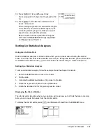
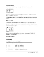
6. Press
o
to display the Y= editor.
If necessary, press
‘
to clear the function
Y1
.
As necessary, press
}
,
Í
, and
~
to turn off
Plot1
,
Plot2
, and
Plot3
from the top line of the
Y= editor (Chapter 3). As necessary, press
†
,
|
,
and
Í
to deselect functions.
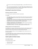
7. Press
y ,
1
to select
1:Plot1
from the
STAT PLOTS
menu. The stat plot editor is
displayed for plot 1.
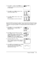
8. Press
Í
to select
On
, which turns on plot 1.
Press
† Í
to select
"
(scatter plot). Press
† y d
to specify
Xlist:L1
for plot 1. Press
† y e
to specify
Ylist:L2
for plot 1. Press
† ~ Í
to select
+
as the
Mark
for each data
point on the scatter plot.
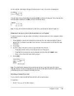
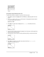
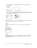
9. Press
q
9
to select
9:ZoomStat
from the
ZOOM
menu. The window variables are adjusted
automatically, and plot 1 is displayed. This is a
scatter plot of the time-versus-length data.
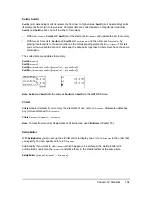
10. Press
… ~
4
to select
4:LinReg(ax+b)
(linear
regression model) from the
STAT CALC
menu.


