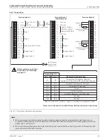


Single and Dual Input Analyzers for Low Level Conductivity
AX410, AX411, AX413, AX416, AX418, AX450, AX455 & AX456
Appendix A
IM/AX4CO Issue 11
73
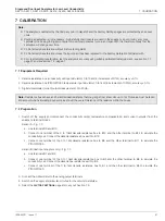
Appendix A
A.1 Automatic Temperature Compensation
The conductivities of electrolytic solutions are influenced
considerably by temperature variations. Thus, when significant
temperature fluctuations occur, it is general practice to correct
automatically the measured, prevailing conductivity to the value
that would apply if the solution temperature were 25ºC, the
internationally accepted standard.
Most commonplace, weak aqueous solutions have temperature
coefficients of conductance of the order of 2% per ºC (i.e. the
conductivities of the solutions increase progressively by 2% per
ºC rise in temperature); at higher concentrations the coefficient
tends to become less.
At low conductivity levels, approaching that of ultra-pure water,
dissociation of the H
2
O molecule takes place and it separates
into the ions H
+
and OH
-
. Since conduction occurs only in the
presence of ions, there is a theoretical conductivity level for
ultra-pure water which can be calculated mathematically. In
practice, correlation between the calculated and actual
measured conductivity of ultra-pure water is very good.
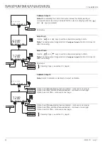
Fig. A.1 shows the relationship between the theoretical
conductivity for ultra-pure water and that of high purity water
(ultra-pure water with a slight impurity), when plotted against
temperature. The figure also illustrates how a small temperature
variation considerably changes the conductivity. Subsequently, it
is essential that this temperature effect is eliminated at
conductivities approaching that of ultra-pure water, in order to
ascertain whether a conductivity variation is due to a change in
impurity level or in temperature.
For conductivity levels above 1
μ
S cm
-1
, the generally accepted
expression relating conductivity and temperature is:
Gt = G25 [1 +
∝
(t - 25)]
Where:G
t
= conductivity at the temperature tºC
G
25
= conductivity at the standard temperature
(25ºC)
∝
= temperature coefficient per ºC
At conductivities between 1
μ
S cm
-1
and 1,000
μ
S cm
-1
,
∝
lies
generally between 0.015/ºC and 0.025/ºC. When making
temperature compensated measurements, a conductivity
analyzer must carry out the following computation to obtain G
25
:
G
25
=
However, for ultra-pure water conductivity measurement, this
form of temperature compensation alone is unacceptable since
considerable errors exist at temperatures other than 25ºC.
At high purity water conductivity levels, the
conductivity/temperature relationship is made up of two
components: the first component, due to the impurities present,
generally has a temperature coefficient of approximately
0.02/ºC; and the second, which arises from the effect of the H
+
and OH
-
ions, becomes predominant as the ultra-pure water
level is approached.
Consequently, to achieve full automatic temperature
compensation, the above two components must be
compensated for separately according to the following
expression:
G
25
=
+ 0.055
Where:G
t
= conductivity at temperature tºC
G
upw
= ultra-pure water conductivity at temperature
tºC
∝
= impurity temperature coefficient
0.055 = conductivity in
μ
S cm
-1
of ultra-pure water at
25ºC
The expression is simplified as follows:
G
25
=
+ 0.055
Where:þG
imp
= impurity conductivity at temperature tºC
The conductivity analyzer utilizes the computational ability of a
microprocessor to achieve ultra-pure water temperature
compensation using only a single platinum resistance
thermometer and mathematically calculating the temperature
compensation required to give the correct conductivity at the
reference temperature.
G
t
[1 +
∝
(t – 25)]
G
t
– G
upw
[1 +
∝
(t – 25)]
G
imp
[1 +
∝
(t – 25)]


