A.
Fitting Functions
A.
Fitting Functions
A.1.
Gaussian
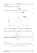
The mathematical description for a Gaussian pulse is:
G
(
t
) =
e
−
t
2
(A.1)
The autocorrelation of this pulse is given by the solution of the convolution integral
G
ACF
(
τ
) =
Z
∞
−∞
G
(
t
)
G
(
t
−
τ
)
dt
=
r
π
2
e
−
τ
2
2
(A.2)
Figure A.1.: Gaussian function
e
−
t
2
and its normalized autocorrelation
e
−
τ
2
2
(dotted line)
Equating the normalized Gaussian functions with
1
2
gives the time value at half amplitude.
G
(
a
) =
1
2
⇒
a
=
p
ln
(
2
)
(A.3)
G
ACF
(
b
)
r
2
π
=
1
2
⇒
b
=
p
2ln
(
2
)
(A.4)
The quotient of these time values supplies the transformation factor between the pulse width and
the FWHM value of its autocorrelation function.
a
b
=
p
ln
(
2
)
p
2ln
(
2
)
=
0
.
71
(A.5)
Pulse
Scout2 Version 1.1
48
July 2015

