


Installation Procedure
ComTec GmbH
2-13
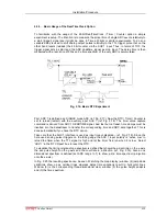
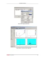
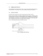
2.5.3. Basic Usage of the RealTimeClock Option
To familiarize with the usage of the 48 bit RealTimeClock / Timer / Counter option a simple
experiment is setup. The intention is to measure the arrival time of single ADC events relatively to
a start (trigger) signal like it might be done in Time-of-Flight or similar experiments. To do so a
variable delay is used to shift analog output pulses relatively to the TTL trigger pulse that on the
other hand resets (reloads) the 48 bit counter via the AUX 1 input. Thus, in terms of TOF, the
trigger signal acts as start and the ADC deadtime signal as stop input. The delay time is then
measured with a resolution of 50ns and a time spectrum of the very ADC is accumulated.
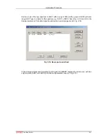
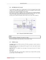
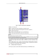
First, ADC 1 is defined as a SINGLE mode ADC (ref. Fig. 2.17). Now the RTC / Timer / Counter is
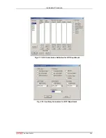
set to reload (restart) with the auxiliary input AUX 1 (ref. Fig. 2.18). The timer value capture
command is derived from ADC 1 DEADTIME signal. And last but not least, time stamps must be
inserted into the datastream to transfer the corresponding time and ADC data together. This is
done automatically if you have the RTC option.
Take care that the AUX 1 interface is used as input (ouput disabled – ref. Fig. 2.18). Since the
here used analog pulser triggers on the falling edge the AUX 1 input polarity is '
active Low
' to
reload the timer when the TTL signal is high and let the timer free run when it is low. Select
'
AUX1
' in the 'RTC Reset‘ box to reset the RTC.
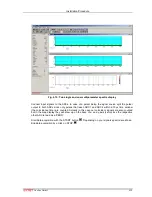
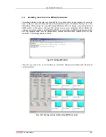
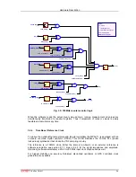
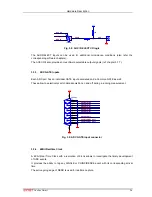
To visualize the timing relationship a spectrum is defined that shows the arrival time on the x-axis,
the adc pulse height on the y-axis and the countrate in z-direction (ref. Fig. 2.19). Also a one
dimensional spectrum is defined (set ADC range to 1) to show just a time spectrum (projection
onto the x-axis).
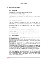
In Fig. 2.20 the resulting spectra can be seen. Watching the map display (window (4)) amplitude
variations show up as vertical lines whereas delay time variations result in horizontal lines.
Window (6) is the corresponding three-dimensional view, window (5) the pulse height analysis
and (3) the time spectrum.
Fig. 2.16: Basic RTC Experiment