Lambda SR1, Operation Manual, Page: 128 / 317

SR1 Operation Manual 128
© 2014 Stanford Research Systems
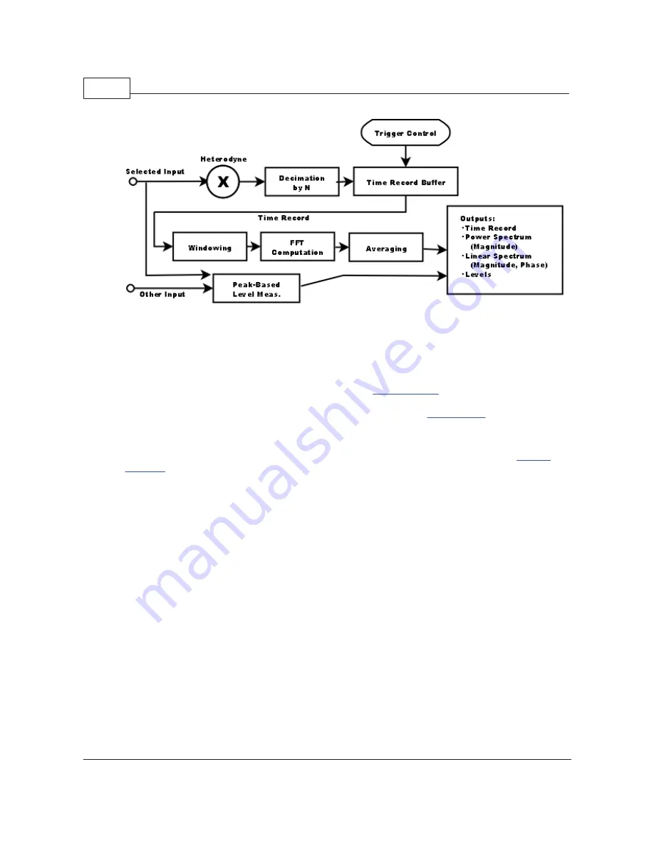
FFT1 Analyzer Block Diagram
A block diagram of the FFT1 analyzer is shown above. The selected input signal is first optionally
heterodyned to move the selected center frequency to the center of the FFT analysis range. The signal
is then optionally decimated by up to a factor of 2
10
in order to reduce the sample rate when using the
"zoom" feature. Each stage of decimation includes filtering to eliminate alias effects from the discarded
portions of the frequency spectrum. The output is sent to a buffer which serves as the time record for the
FFT analyzer. Each time record starts with a trigger. If the
analyzer trigger is not enabled then a trigger
is automatically generated as soon as the DSP has finished processing the previous time record.
Otherwise, the analyzer waits for a trigger which matches the specified
trigger criteria and begins the
time record at the trigger point.
After a trigger occurs and enough time record points have been accumulated to compute a spectrum of
the specified resolution, the DSP applies a windowing function to the time-domain data (See
Window
Selection ). Windowing is necessary due to the finite length of the FFT time record. Unless the input
signal happens to be periodic in the time record, discontinuities at the beginning and end of the time
record will appear as significant broadening of the true spectrum of the input signal. Window functions
are large in the middle of the time record and taper off at the beginning at the end in order to minimize
the offending discontinuities.
After windowing, the DSP computes the FFT of the windowed time record. For a resolution of N lines, 2N
real time record points are used to compute an FFT of N complex points. Each FFT is then averaged in
two different ways. The
Power Spectrum is computed by computing the power for each spectrum
(taking the absolute value of the complex FFT points) and averaging that power into the power computed
for previous FFTs. This type of averaging does not reduce the noise floor of the spectrum but it does
reduce the variation of the noise floor making it easier to see spectral details on the order of the noise
amplitude. Phase information is lost when computing the Power Spectrum. In the example below, the
unaveraged power spectrum is shown for a signal composed of a 1 kHz sine wave with added white
noise. The second spectrum shows the power spectrum with averaging on and Navg = 10. Note the
substantial reduction in the variation of the noise floor and note also that the average value of the noise
floor is is the same in the two spectra.