20
To save data as an image (flattened or not), the user will open the main File menu in the software,
and click on “Save Graphics”.
This opens a Save Graphics File window (Fig 15), where the user can
define the size of the image, choose the file extension from a drop down menu (including JPEG and
TIFF), and in
dicate a file name and path. Click “Do It” to execute.
Alternatively, from the data window,
clicking on “Command” opens a drop down menu with an option to export the file as a TIFF. This drop
down menu also has the option to toggle between a “classic” and “new” appearance, which may be
helpful to meet the formatting demands of a technical journal or a PI.
To analyze the sample surface, click on the A button in the data window. This opens the Analyze panel
to the “Roughness” tab
(Fig 16b).
The fields are automatically populated with surface roughness data
related to the full image. The user can define a box-shaped mask to calculate roughness of a box-shaped
subsection of the image. The “Section” tab of this window allows the user to draw a line on the data
image, and the software will calculate the length of the line, or cursors may be dropped on the line in
order to measure a subsegment of the line. The line is a minimum of one pixel thick, but the user may
make the line thicker in order to average more data points on the line.
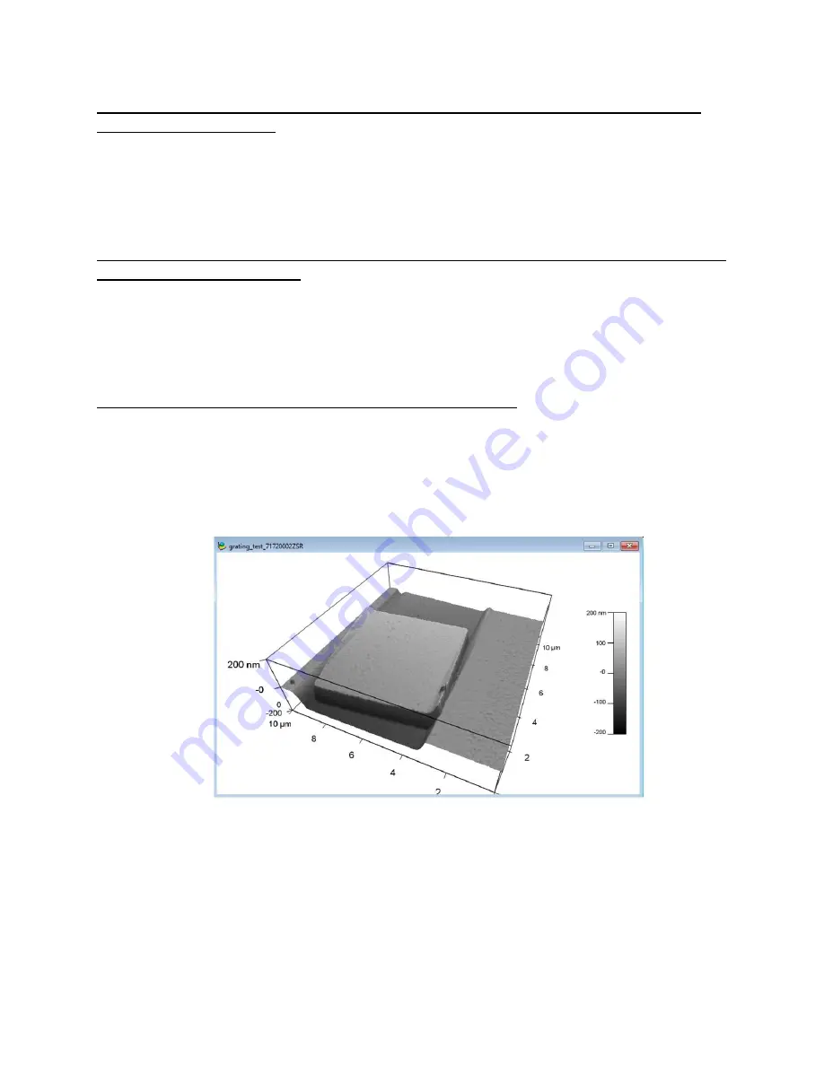
To see a 3D plot of the data, click the 3D button on the data window
. This opens a new window with a
3-dimensional rendering of the data with scales on the x-, y-, and z-axes (Fig 17). The user may click on
the image and drag to rotate and view the rendering from other angles. This image can be saved and
exported to a JPEG or TIFF as previously discussed.
Figure 17. An image of a 3D rendering of data


