


The above example shows how the ECAM program is structured and how the commands can be
given to the controller. The next page provides the results captured by the WSDK program. This
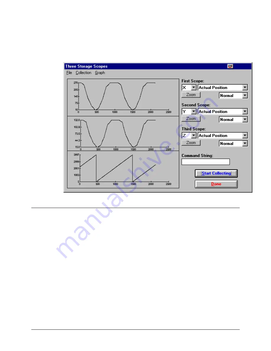
shows how the motion will be seen during the ECAM cycles. The first graph is for the X axis, the
second graph shows the cycle on the Y axis and the third graph shows the cycle of the Z axis.
Figure 6.5 – WSDK program results – Three Storage Scopes
Contour Mode
The DMC-1600 also provides a contouring mode. This mode allows any arbitrary position curve
to be prescribed for 1 to 8 axes. This is ideal for following computer generated paths such as
parabolic, spherical or user-defined profiles. The path is not limited to straight line and arc
segments and the path length may be infinite.
Specifying Contour Segments
The Contour Mode is specified with the command, CM. For example, CMXZ specifies
contouring on the X and Z axes. Any axes that are not being used in the contouring mode may be
operated in other modes.
A contour is described by position increments which are described with the command, CD x,y,z,w
over a time interval, DT n. The parameter, n, specifies the time interval. The time interval is
defined as 2
n
ms, where n is a number between 1 and 8. The controller performs linear
interpolation between the specified increments, where one point is generated for each millisecond.
Consider, for example, the trajectory shown in Fig. 6.4. The position X may be described by the
points:
DMC-1600
Chapter 6 Programming Motion
•
95


