enabling
innovative
electronics
Ossila Ltd
Copyright © 2009-2015
76
Example:
Let us suppose that a TC curve is acquired for Gate voltages ranging from 0 to -80 V at a
constant Drain voltage of -60 V, where the transistor is operating in Saturation mode. Let also
suppose that the drain current is measured for any voltage change, i.e. ΔV
GS
=1V, and that
N
, the size
of the data subset, is set equal to 10.
When the measurement is completed, the TC data set is then represented by 81 couples (
V
GS,i
,
I
DS,i
),
with
i
index labelling the input/output couples. The first couple, (
V
GS
,0
=0
,
I
DS
,0
) is discarded, while the
rest of the data is organized in ten-point subset. The first subset is formed by the gate voltages (-1, -
2, -3, ..., -9, -10) V and the respective measured currents. The second one is composed by the gate
voltages (-11, -12, -13, ..., -19, -20) V with the current measured at these gate voltages and so on. For
each subset, the linear fit is calculated and its slope is used to calculate the mobility through Eqs. 4
and 9. The motilities so obtained, are then plotted as function of the average gate voltage for each
subset, which in these example are -5.5 V, -15.5 V, -25.5 V, and so on up to -75.5 V. Figure 27 shows
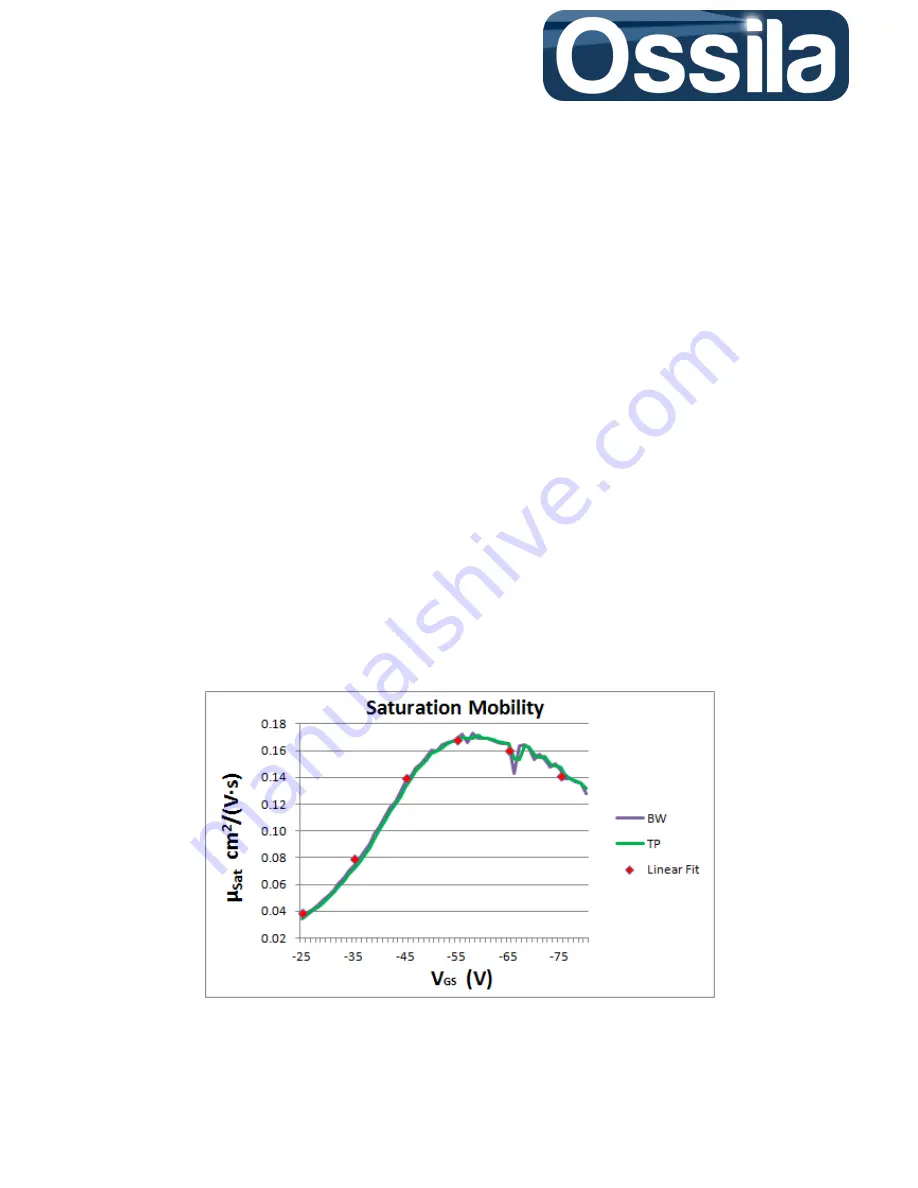
the mobility calculated with the partition method (using Eq. 9 for each data set) and the derivative
method, Eq. 11. In both case the data are not processed through any filter, so that the effect of the
noise on the derivative can be fully appreciated.
On figure 27 the derivative is calculated using the both backward numerical differentiation (BW) and
the more error-robust two-point method (TW), see Eq 30. Since the numerical differentiation
amplifies the measurement uncertainty (noise), the resulting mobility curve can be non-smooth and
“noisy”. On the other hand, the modified linear fit method extrapolates the mobility over ten data-
point set and is therefore intrinsically more robust against measurement noise while still providing
the correct gate voltage dependence of the mobility.
Figure 27. Comparison between the field effect saturation mobility calculated from the modified
Eq. 9 (Linear Fit), (BW, TP) using two different numerical derivative methods. For each data set,
the saturation mobility is plotted as function of the mid-point interval

