Adaptive® JUNIOR – Technical and HMI User Guide
REV 1.04
19
When the auto tune completes successfully the P, I and D
gain terms will be automatically updated with the results
and the control mode will swap to PID. Figure 19 shows
the plot after tuning, you can see the end of the last tuning
cycle and then the transient to the new setpoint value.
The system should now be tested for transient response
and at the expected extremes of the system range to
ensure it remains stable at all times. The tuning results can
now be used as a starting point for finer tuning to increase
system performance.
Warning:
As an algorithm is being used to perform the auto tune and cannot be exposed to all the disturbances or
adjustments possible, it is up to the user to confirm the tuning is suitable.
Over temperature, under temperature
and over current alarms should always be employed in the system to ensure adequate protection to the user and
equipment from oscillatory or prolonged full-scale outputs.
4.5.5.
PID Basics Explained
The PID control method works by first calculating the error between the actual and desired temperature (setpoint –
sensor D feedback). This error is then multiplied by the P (Proportional) gain value to give an output that is
proportional to the error. This output will reduce the resulting error and so on. However, this has a limitation as there
must be an error present to produce an output to maintain the temperature. The larger the drive that is required the
larger the error is needed to produce it. The P gain could be increased to reduce the error but repeatedly doing so will
eventually cause the system to oscillate as the output is driven strongly on the small errors. Proportional control will
give output that will overshoot the setpoint and always remain short of the desired temperature. It is not suited to
situations that have large variations in the load.
The I (Integral) term is used to reduce the remaining error left by the P term. It does this by accumulating the error
over time (integrating) and adding the result to the output. As the temperature reaches the setpoint and the error
becomes too small to have any effect on the P term the I term becomes dominant and continues to reduce the error
to zero. Although this results in little or no error it comes at the cost of speed as the system response is reduced.
The final option to control the output is to look at the change of the error over time, this is the Differential and it is
adjusted using the D term. When the error isn’t changing much the output from this term will be low, however if
there is sudden disturbance or the setpoint is adjusted the resulting error will change sharply. This large change over
a short period will provide a strong output to quickly move the temperature, and as the temperature starts to move
towards the setpoint the rate of change will start to reduce, reducing the output drive. This has the effect of being
able to quickly respond to changes without overdriving the output as the error reduces.
Tuning a system is finding the right combination of PI or PID values that produce the best response. For example, too
much P will give overshoot, too large I will reduce the response speed and too much D will amplify any noise present
in the system. Incorrect values will also lead to instability and oscillation of the temperature around the setpoint.
Figure 19 End of Auto Tune sequence


