


28
AQUA M A STE R4
|
EL EC T R O M AG N E T I C FLO W M E T ER I N SER T I O N SEN S O R | O I/FE W4 0 0/A P - EN R E V. B
…Appendix
Velocity profiles background
The Point of Mean Velocity is on the knee of the curve (the
velocity at this point is changing rapidly with distance) so it is
necessary to position the insertion sensor extremely accurately
in order to measure the correct velocity. If the insertion sensor
is inserted accurately to 72.5 mm, it is therefore measuring the
mean velocity of 1.722 m/s which, when multiplied by the area,
gives a volume flow of 487 l/s. If the insertion sensor is inserted
to 74 mm instead of 72.5, the velocity measurement is 1.85 m/s
instead of the expected 1.722. Multiplying this figure by the
area results in a volume flow of 523 l/sec – an error of 7.4 %.
On-site it can be very difficult to locate a insertion sensor
exactly, so this sort of error is quite common. With insertion
sensors other than this insertion sensor, working under any
degree of pressure in the line, inserting a insertion sensor to
within 10 mm of its intended location is often accepted. Using
the calculation above, this produces an error of approximately
15 %. This can be reduced significantly by using the following
method.
Referring to Figure 28, in the middle of the pipe, near the center
line, the profile is relatively flat, i.e. the flow velocity does not
change very much with distance into the pipe. Therefore, if the
velocity is measured on the center line, measurement errors
due to positional errors (i.e. not locating the insertion sensor
where required) are very small; hence most users will try to use
the center line measuring position. However, as explained
previously, this process gives us the wrong answer, Fortunately
there is a mathematical relationship between the velocity at the
center line and the mean velocity within the pipe – the Profile
Factor (F
ρ
).
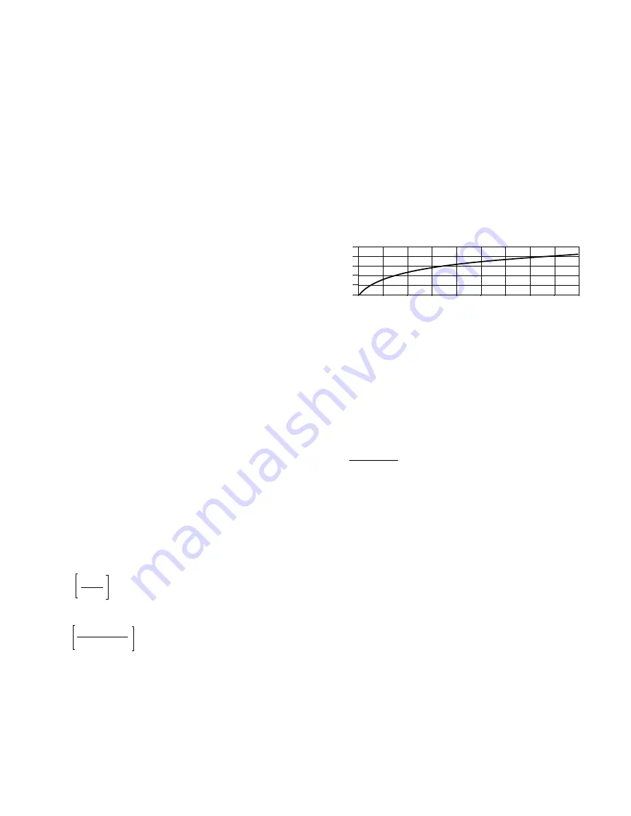
The value of F
ρ
can be calculated by an equation (below) or
obtained from a graph – see Figure 29.
F
ρ
is calculated as follows:
where:
and:
n = 1.66log(Re)
and:
D
Re =
–
ρν
µ
key
:
D = pipe diameter
ρ
= fluid density
ν
= average fluid velocity
µ
= fluid viscosity
Pipe bore in mm
Pipe bore in inches
P
ro
fi
le f
ac
to
r (
F
p
)
200
400
600
800
1000
1200 1400
1600
1800
2000
8
0.875
16
24
32
40
48
56
64
72
80
0.870
0.865
0.860
0.855
0.850
Figure 29 Profile factor vs flow velocity for pipe sizes
200 to 2000 mm (8 to 78 in)
When the insertion sensor insertion position is determined, the
effect of putting the insertion sensor into the pipe (see page
27) must be calculated.
The blockage or insertion effect is termed the
Insertion Factor
(Fi)
. This is a mathematical relationship and can be calculated
from the formula:
Testing the flow profile for symmetry
If there is any doubt as to the symmetry of the flow profile (see
page 10), a Partial Velocity Traverse must be carried out.
This procedure involves comparing the value of velocity at two
points at equal distances from the center line.
It is normal to compare the flow velocities at insertion depths
of 1/8 and 7/8 of the pipe diameter as these points are always on
the 'knee' of the profile.
Partial velocity traverse
Determine the internal diameter D of the pipe, in millimeters, by
the most accurate method available. If the insertion sensor
insertion length is greater than the internal diameter of the
pipe, proceed with the Single Entry Point Method. If the
insertion sensor’s insertion length is less than the internal
diameter of the pipe, proceed with the Dual Entry Point
Method.
F 1
(r – Yb)
r
=
–
–
1
n
ρ
Y
b
r
(n + 1) (2n + 1)
2n
=
2
F
i
=
1
1 – (38/(
π
D))


