MicroE Systems Dual Axis Averager Mercury 3000Si, Инструкция по установке и справочник

Страница: 25 / 27

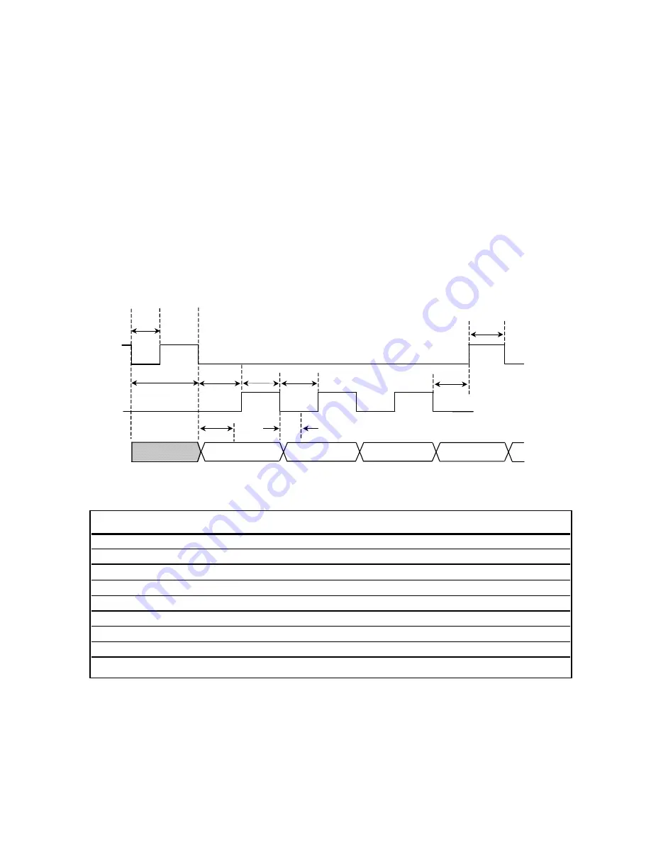
Operational Modes: Trigger Approach Timing Diagram
Symbol Parameter Minimum Typical Maximum Units
tspiH spiClock High Time 50 ns
tspiL spiClock Low Time 50 ns
tTDR n
_
spiEndable to DataReady 1420 1600 ns
tW n
_
spiEnable Low for trigger 50 ns
tCSC n_spiEnable to spiClock 0
tCSD n_spiEnable to DataValid 80 ns
tV spiClock to Data Valid 80 ns
tCCS spiClock to n_spiEnable 0 ns
tCS n_spiEnable High 50 ns
Trigger Approach Timing Diagram
The Trigger Approach can be used in applications where synchronization of the position data to an event is required. Often, this
mode is used when a fixed latency between a clock signal and the sampled position data is required. The customer can choose
this mode of operation by using the optional SmartPrecision Software. In this mode, triggering is controlled by the n_spiEnable
signal.
The falling edge of n_spiEnable signal starts the process by immediately resetting the internal calculators and acquiring the latest
A/D converter information. Old data in the calculation chain is discarded and the initiation of a new position calculation is started.
The new data is ready in 1420ns. The n_spiEnable signal for retrieving the data must be asserted within 210ns after the new data
is ready or the triggered acquisition will be over written by new data.
Shifting the data out of the interpolator's serial port is accomplished exactly as in the Standard Communication mode of operation.
In order to sample the next position, n_spiEnable must be brought high and then reasserted. See the Trigger Approach timing dia-
gram below.
tV
Clk1 Clk36
MSB LSB
n_spiEnable
spiClock
spiDataOut
tTDR
tW
tspiH tspiL tCSC
tCSD
tCCS
tCS
Trigger Approach Timing Diagram
Page 23