6
(displayed in the pressure
coordinate field) is
locally minimal.
Select/Deselect with
space key. In Coach 6
you can maximize the
Select/ Remove dialog.
5.
Mark
Keep selected
and
click
OK
. As the result
you get circa 25 points of
the lower part of the
envelope curve. These
points determine the
graph of the trend
pressure. To get a
smoothed graph with the
number of points of the
original graph through
these points you are going to use the Spline function. Select the option
Process >
Smooth
.
6.
Select as Function Type
Spline
. Type the original number of points (determined in step
1) in the Number of Points field. Leave all other settings as they are. Mark
Replace
data
and click OK. The calculations may take some time.
7.
Rename the pressure quantity p to ‘p-trend’.
8.
Save the results under the new name ‘Trend pressure’ by using the option
Save as…
.
Determination of upper pressure values
1.
Open the original measurement
results.
2.
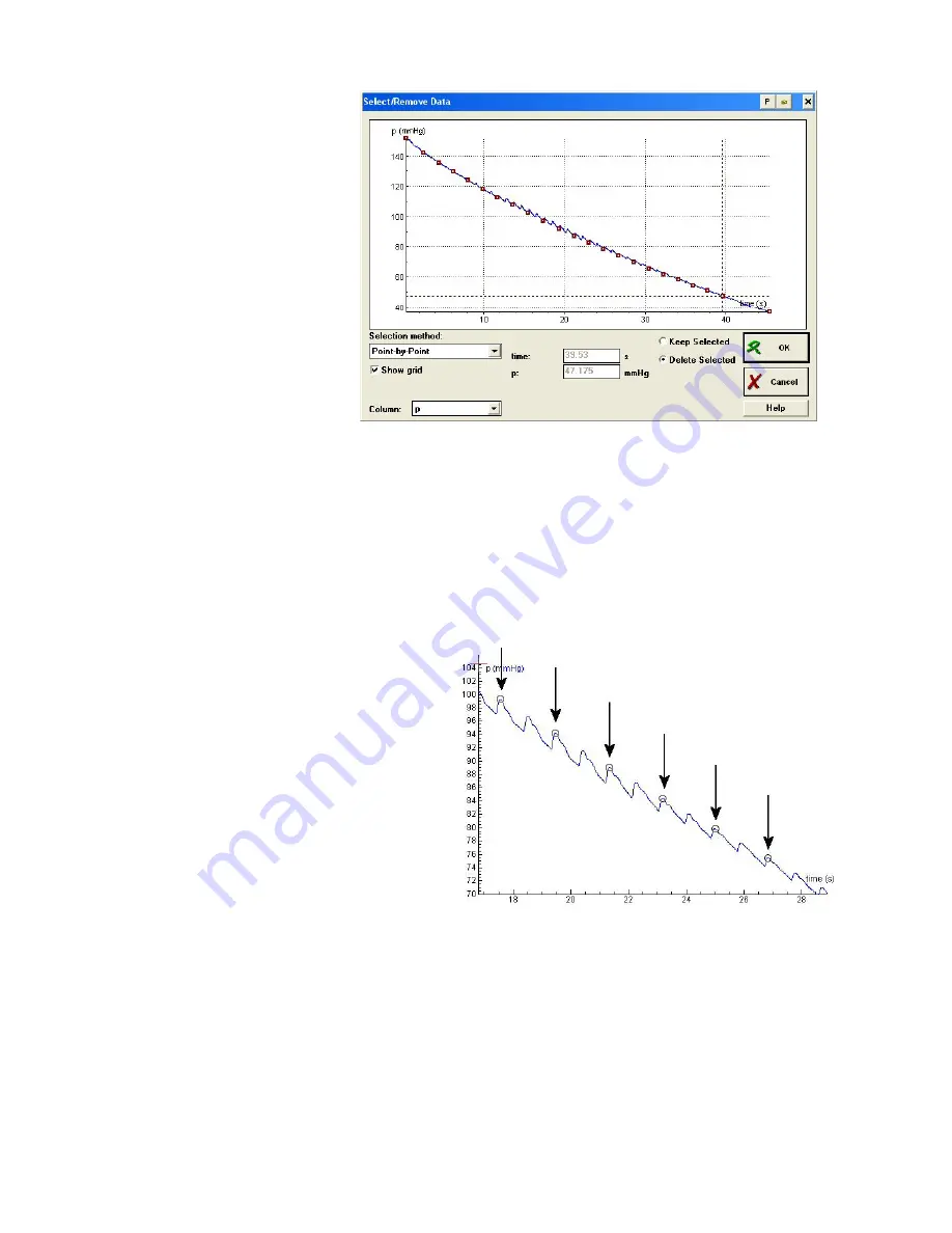
Repeat the steps 2 to 6, but this time
mark the maximal pressure values, the
tops of the pulses.
It is enough to mark every second
maximum (see the figure 7).
3.
Rename the pressure quantity to ‘p-
pulse’ and save the results as ‘Pulse
pressure’.
Determination of the envelope curve
You have now two result graphs from
which the difference graph should be made.
1.
Open the original measurement result. Place the measurement table in one of the Coach
panes.
2.
Select in the Table menu the
Import data > Coach Junior/Coach 5 Result
option.
3.
Select in the dialog the result ‘Pulse Pressure’.
4.
In the Import data dialog column C1 is selected in the Original data part, select in the
Import as part ‘Column: none’.
5.
Click column C2 in the Original data part and set in the Import as part ‘Column: C3’.
Figure 5.
Selection of circa 25 cuff pressure points.
Figure 7.
Selection of the upper pressure points.


