


2DH Boussinesq Wave Module - Examples
77
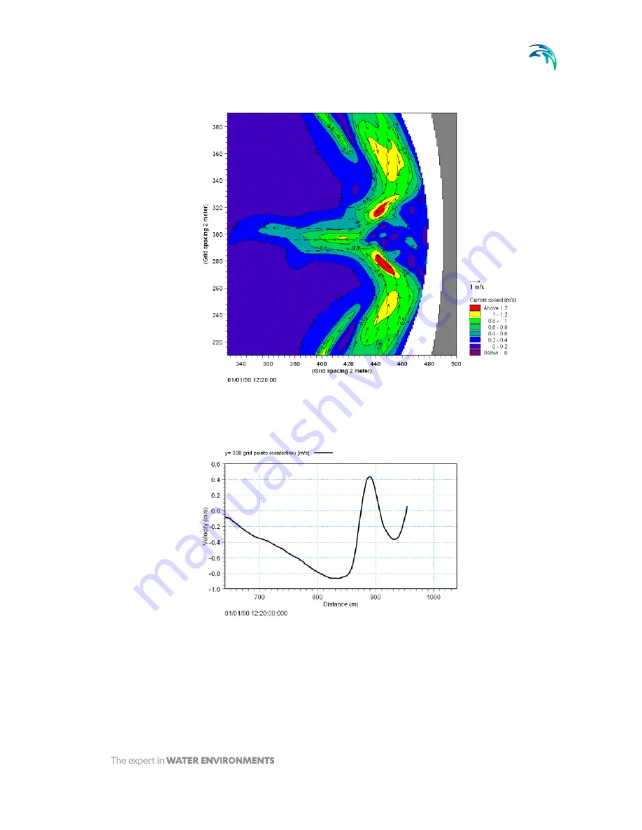
Figure 4.47
Depth-averaged wave-induced current focusing on the symmetrical cir-
culation cell
Figure 4.48
Rip current along the rip channel (y= 300 grid points)
The rip current significantly affects the wave motion. The large variation of the
rip current causes an increase in the wave height, which can be seen in
Figure 4.46 (lower panel). The rip current also causes a small local bend in
the wave crest occurring at the centre line as observed by Hamm.
Summary of Contents for 21 BW
Page 1: ...MIKE 2017 MIKE 21 BW Boussinesq Waves Module User Guide...
Page 2: ...2...
Page 4: ...4 MIKE 21 BW DHI...
Page 16: ...Introduction 16 MIKE 21 BW DHI...
Page 190: ...Reference Manual 190 MIKE 21 BW DHI...
Page 192: ...Scientific Documentation 192 MIKE 21 BW DHI...
Page 193: ...193 INDEX...