


Manual, Ultra High Sensitivity Aerosol Spectrometer (UHSAS)
DOC-0210 Rev E-4
3 0
© 2017 DROPLET MEASUREMENT TECHNOLOGIES
6)
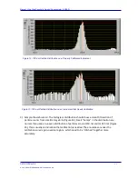
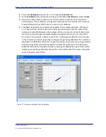
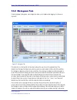
Once the process stops, the graph should show the data points scattered around a best-
fit line.
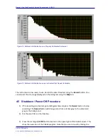
7)
Repeat this procedure for the other relative gain tabs, which are labeled
G2:G1 Gain
and
G1:G0 Gain
. Acquiring a sufficient number of large particles (for G1:G0) may take up
to ten minutes, especially at flow rates below 60 sccm.
Note:
The program will
automatically use the new gain and offset parameters as long as the current session is
running; however, if these parameters should be used permanently, they must be saved
in the configuration file. To do this, click on the
Save
button on the
Configuration
tab.
Several comments on the relative gains are needed. In the particle-size regions where detection
passes from one gain stage to another, there can be discontinuities in the histograms produced.
The histograms are very sensitive to the relative gain parameters, which are experimental
quantities subject to statistical and systematic error. The stitching region between G2 and G1 is
particularly prominent in this regard, since the detection technique changes between these gain
stages—they are physically different photo-detectors. The ability to study these transition
regions with high resolution can overemphasize the stitching errors. In most cases, the semi-
auto-calibration provided should be adequate.
Stitching errors between the gain stages will be more noticeable for certain choices of bin map.
This is the case if, near the stitch region, the bin width is less than 1% of the bin center. For
instance, say a bin in a stitch region collects 299-301 nm particles. In this case, the bin width (2
nm) is less than 1% of its center (1% of 300 nm, or 3 nm), so stitching errors may occur.
5.2.3
Step Two: Absolute Calibration
1)
Gather a collection of particles to be used as reference particles. Recommended sizes
are 100 nm, 269 nm, 500 nm, and 930 nm. Using all four of these sizes will test all the
instrument’s gain stages. The instrument can also be tested with just 100 nm particles
or with 100 nm and 930 nm particles, but the results will not give as clear a picture.
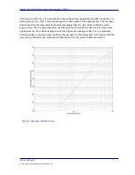
2)
Click on the
Calibration curve
tab. The current calibration curve should be shown.
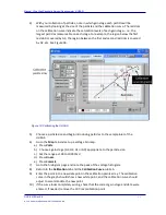
3)
Clear all data from the calibration points array (see Figure 18) EXCEPT for the 100-nm
point on gain stage. To clear a data point, right-click in the cluster box that contains
the three point values (Gain, mV, nm) and select
Delete Element
.
Note:
The points
array displays one point’s information at a time. To see a new point, click on the
arrows above the
Points
label. The
Points
field shows the element in the points array
that is currently displayed.


