


have been entered. If you have changed the recording
parameters, the arrow will flash yellow-green. After you finish
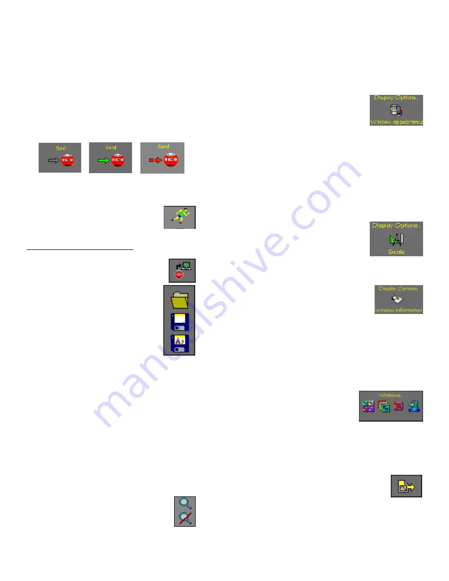
setting all the parameters in the panel, press the flashing Send
icon.
If the settings are downloaded properly to the OaktonLog device,
the Send arrow stops flashing and returns to the default wire-
frame mode. If the icon changes to a broken red arrow, the
settings have not been saved in the OaktonLog. Make sure the
OaktonLog is communicating with your PC (refer to page 3) and
that it is stopped (refer to page 3).
3 modes of the Send button
No update
needed
Click to update
OaktonLog
No
communication
Starting the Logging Run
After you finish setting up the OaktonLog, it is
time to start the data recording.
Click the
Run
icon on the left toolbar. Once you
click it, The OaktonLog starts recording data,
based on the pre-programmed parameters.
Downloading and Viewing Data
Downloading is done by clicking the
Data
Download
icon on the left toolbar. Make sure that
the OaktonLog's communication port is open.
File management
The three top icons on the left toolbar of MicroLab
are used for file management. Clicking the
Open
icon opens saved files. Clicking the
Save
icon
saves the file you are currently working on. If you
save your results the first time, you have to enter
a file name into a dialog box opening up. The file
name cannot consist of more than 8 characters.
The extension of the data files used by MicroLab
is *.SMP.
The
Save AsÉ
icon is used to save an already
saved data file under a different name.
Viewing the Data: The Markers
The MicroLab software supplies you with a helpful marker tool.
The marker is used to view the data at a specific moment, or to
measure the difference between two points in the graph.
To place a marker on the graph, double-click on the desired place
on the graph. A black arrow appears on the graph, and at the
bottom of the graph window the Y and t values represented by the
marker appear. You can move the marker by placing the mouse
pointer on it, holding the left mouse button, and dragging the
marker to the left or right. You can also place the mouse pointer
on the marker, left-click once, and then move the marker by using
the left and right Arrow keys on your keyboard.
Placing a second marker is done the same way. When you place
the second marker, the data at the bottom of the window include
the values for
∆
X,
∆
t.
∆
refers to the difference values between
the markers.
To remove a marker, click on it with the right mouse button.
Viewing the Data: Zooming
Zooming in is done by clicking the
Zoom
icon on the
left tool bar. Once clicked, the mouse pointer changes
to a magnifying glass. Place it on the beginning of the
section you wish to zoom in, press and hold the left
mouse button, and drag the mouse pointer over the section you
wish to zoom in. Once released, the window displays only the
zoomed data. Pressing the right mouse button will zoom the plot
out to the previous position. If you wish to view the original data,
click the
Full view
icon. Clicking anywhere outside the graph
window will turn the mouse pointer back to
its normal mode.
Viewing the Data: Display Options
On the left tool bar you can see a screen
icon. When the mouse pointer is placed on
it, the Display options sub-menu opens.
You can select one of three options
Window Appearance
Ð Your mouse pointer changes to a brush.
Placing the brush on one of the graphs or on the background of
your data window and clicking there with the left mouse button
opens a color dialog box, in which you can select a different color
for graphs or background.
Clicking on one of the data graphs with the right mouse button
opens the Line preferences dialog box, where you can select line
type, line width, and a symbol to be placed where the data points
were recorded.
Placing the brush on the X or Y-axis of your graphs, or on the
graph title, opens the Font dialog box, in which you can select the
font type, size and color for the axis and
the main title.
Viewing the Data: Scaling
Scaling means changing the minimum and
maximum values of your graphÕs Y-axis.
Clicking the Scale icon with the left mouse
button opens the Scaling dialog box. Select the graph you wish to
scale, and enter then the new Min and Max values. Click OK to
apply the scaling on the graph.
Viewing the Data: Window information
Clicking the
Window information
icon with
the left mouse button will turn the mouse
pointer into a notepad. Placing it on a graph
and clicking it opens the Information window
of that graph, where you can see or change the graph's name, or
enter a title for the graphÕs Y-axis, and view the applied sensor
and start time for that graph.
Placing the notepad mouse pointer clicking on the window title
with the left mouse button opens the Information window, where
you can change the title of the window, enter a title for the X-axis,
and view the sensor and the total number of samples taken. In
both of the dialog boxes, the mouse pointer returns to its normal
mode upon clicking OK. If you wish to continue using the notepad
mouse pointer, click ÒSee More InfoÓ.
Viewing the Data: Windows
Arrangement
On the bottom of the left toolbar, you
find the Windows submenu. Place the
mouse pointer on the icon to see the
options for arranging the windows:
Tile
Ð Displays all open windows next to each other so that they
fill the MicroLabÕs work area.
Cascade
Ð Alters all open windows so that they all have the same
size, and arranges them in a cascading fashion on the top at the
left side of the screen.
Close all
Ð Closes all open windows.
Exit
Ð Exits MicroLab.
Viewing the Data: Output Options
Placing the mouse pointer on the output icon in the
left toolbar displays the output options of the MicroLab software.
There are 3 output options:


