Kaco 1001202, Руководство пользователя, Страница: 62 / 93

Fig. 47: Equation 1
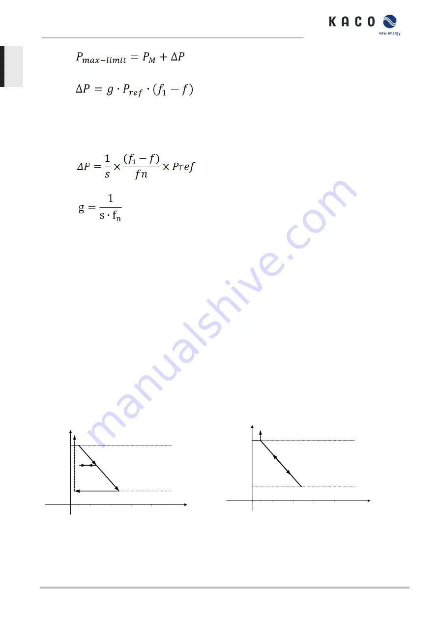
Fig. 48: Equation 2
Gleichung 1 [See figure 47 [ } Page 62] definiert die maximale Grenze mit ΔP entsprechend Gleichung 2 [See
figure 48 [
}
Page 62], P
M
die Momentanleistung zum Zeitpunkt der Aktivierung und P
ref
die Referenzleistung.
In the case of PV inverters from KACO, P
ref
is defined as P
M
, the current power at the time of activation. f is the
current frequency and f
1
is the specified activation threshold.
Fig. 49: Equation 3
Fig. 50: Equation 4
In some standards, the power adjustment is specified by a drop (s) instead of a gradient (g), as shown in equa-
tion 3 [See figure 49 [
}
Page 62]. The drop s can be transformed into a gradient g in accordance with equation
4 [See figure 50 [ } Page 62].
The frequency f remains above the activation threshold
f
1
during an overfrequency incident. Consequently, the
expression (
f
1
–
f
) is negative and ΔP corresponds to a reduction in the feed-in power.
The measurement accuracy of the frequency is greater than 10 mHz.
The specific mode of operation of the function is specified by the grid operator or the pertinent standards or
the grid connection guidelines. The configurability of the function makes it possible to satisfy a wide variety of
standards and guidelines. Certain configuration options are not available in some country settings because the
pertinent standards or grid connection guidelines prohibit adjustments.
Adjusting the active power P(f) in the event of underfrequency
Some grid connection guidelines also require adjustment of the active power P(f) in the event of underfre-
quency. Due to the fact that PV systems are typically run at the maximum power point, there are no power re-
serves for increasing the power in the event of underfrequency.
However, in the event that the system power is reduced due to market regulation, it is possible to increase the
active power up to the power level available. Because the inverter is unable to distinguish between P constant
target values for obligatory bottleneck management by the grid operator and for market regulation, this needs
to be implemented in the site-specific infrastructure of system control.
52 , 0 51 , 5 51 , 0 50 , 5 50 , 2
100 % P
M
60 % P
M
P
ref
= P
M
P
f P
1
re
=
eff
= =P
e
50
P
,
P
M
P
2
M
Hz f
1
s
1
= =
=
= =5 5
5
50,
% s
f s 5
stop
5% 5
p
=
% %
50 , 1 Hz
Frequency [Hz]
Active Power [%P
Re f
M
=%P ]
Fig. 51: Example behaviour with hysteresis (mode 1)
52 , 0 51 , 5 51 , 0 50 , 5 50 , 2
100 % P
M
60 % P
M
P
ref
= P
M
P
f P
1
ref
=
f
=P
f
50
P
,
P
M M
P
2 Hz f
1
s
=
=
=5 5
5
50,
% s s
f s 5
stop
5 5% %
=
% % % % %
deactivated
Frequency [Hz]
Active Power [%P
ref
M
=%P ]
Rate limited power increase after
deactivation of response
Fig. 52: P(f) example characteristic without hysteresis Mode 2
10 | Specifications Manual
KACO blueplanet 3.0 TL3 KACO blueplanet 4.0 TL3 KACO blueplanet 5.0 TL3 KACO blueplanet 6.5 TL3 KACO
blueplanet 7.5 TL3 KACO blueplanet 8.6 TL3 KACO blueplanet 9.0 TL3 KACO blueplanet 10.0 TL3
Page 62
EN