This can easily be accomplished using two PPT units, one at the pressure point and one by the chart
recorder. A two-wire digital interface would transmit PPT1 pressure information to the PPT2 re-
corder point. The digital RS-232, or RS-485, line is more tolerant of noisy environments and connec-
tor losses than an anaolg signal. Commercially available RS-232, or RS-485, drivers and repeaters
are available to extend the distance between the two PPT units, up to several miles if necessary. The
PPT2 unit can be placed close to the chart recorder with very little, if any, noise on the analog
output. When the RS-232, or RS-485, baud rate is set to 28,800 baud, the reading delay imposed by
the digital transmission is 2 msec. The benefit of using two PPTs this way is that it is quick and easy
to implement and that no software development is required. Using this technique, the RS-232
connections can be configured as a single two-wire bus that accommodates up to nine pairs of PPT
units simultaneously sensing remote pressures. In order to avoid bus collisions on a RS-485 bus only
one pair of PPTs may be operated in this mode.
The PPT units should be configured as follows so that they will begin transmitting and outputting
analog readings when power is applied (see Table 4.1). To connect additional PPT pairs to the RS-232
bus, configure each pair with a unique group number. Nine groups are available from number 90
through 98. The example shown in Table 4.1 assumes both PPT units are in the same group - factory
default group is 90.
Commands to setup PPT1
Commands to setup PPT2
Input
Comment
Input
Comment
*01WE=RAM
Write enable
*02WE
Write enable
*01DA=U
Pressure to ‘~’ format
*02DA=R
Digital to analog output
*01MO=P4
Power up mode
*02NE=DAC
Enable write to DAC
*01WE
Enable EEPROM write
*02WE
Enable EEPROM write
*01SP=ALL
Store all to EEPROM
*02SP=ALL
Store all to EEPROM
Table 4.1—PPT to PPT Remote Sensing Setup Commands
4.9
COMMAND ILLUSTRATIONS
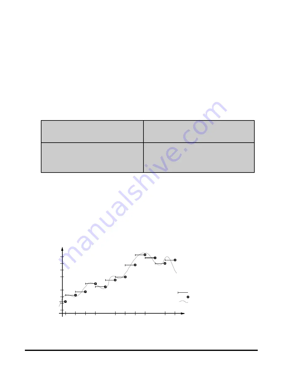
The figures below illustrate the commands that affect the pressure output rate. Figure 4.13 shows a
varying pressure signal having a reading integration time of 200 msec. If the small variations on the
pressure signal are considered noise and are undesirable, increase the integration time to time-
average the pressure signal, and filter out the noise.
5.24
5.20
5.16
5.12
5.08
5.04
5.00
4.96
4.92
Pressure
(psi)
Integration Time
(0.2 sec)
Integration Time = 0.2 sec
(
I
=M2 sets 2x100 msec/sample)
I
= M2
I
C = 0
S2 = 0 S5 = 0
RR = 0 OP=A
Integration time
PPT pressure output
Actual pressure
1.
0
2. 3.
0 0
Time (sec)
Figure 4.13—Integration (I=) Command, Example 1
2 0