THORLABS FSAC, Руководство пользователя

Страница: 18 / 27

Interferometric Autocorrelator Chapter 5: Theory and Interpretation
Page 16
TT121442-D02
is proportional to the input pulse FWHM by the factors in Table 2. Search for “FSAC” at Thorlabs’ website to find a
sample MATLAB or Python script for converting interferometric autocorrelation data to an intensity autocorrelation
trace. The script performs the following functions:
1. Load interferometric autocorrelation data.
2. Load offset data (data taken with laser blocked).
3. Subtract mean offset from interferometric autocorrelation data.
4. Shift time axis data,
t
, so that
t
= 0 corresponds to the peak autocorrelation signal.
5. Determine the fundamental fringe frequency,
f
, from the magnitude of the Fourier transform data.
6. Use the fundamental frequency to convert the time axis,
t
, to a delay axis using the central wavelength of
the input laser,
λ
, and the speed of light,
c
.
Delay f /
7. Set all frequencies outside of
f /2
to zero to remove all fringes.
8. Perform an inverse Fourier transform on the filtered data to get an intensity autocorrelation with background.
9. Using points near the beginning and end of the trace, estimate the background and subtract it from the
intensity autocorrelation trace to get the background free intensity autocorrelation trace.
10. Determine the background-free intensity autocorrelation FWHM.
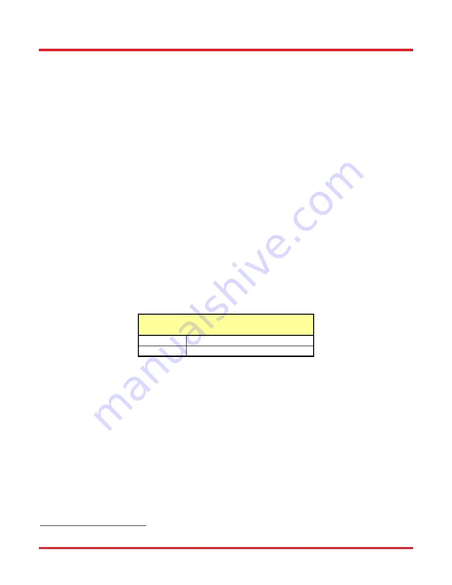
11. Convert to a pulse FWHM by assuming a pulse shape and using the values in Table 2.
Intensity (Non-Interferometric)
Autocorrelation FWHM Relations 3
Gaussian
τ / 1.414
sech
2
τ / 1.543
Table 2
5.4. Excessive Chirp
If the pulse is significantly chirped so that the pulse length greatly exceeds the coherence length of the laser, then
the autocorrelation will appear as in Figure 13. The wings of the autocorrelation are identical to those of an intensity
autocorrelation, and the point at which the trace transitions to an interferometric autocorrelation can be used to
quantify the chirp
4
. In this case, it is not straightforward to interpret the pulse width without additional post-processing
(i.e., filtering out the fringes as described above). See the cited references for more information on interpreting
autocorrelation traces.
3
Diels, Jean-Claude, and Wolfgang Rudolph. Ultrashort laser pulse phenomena. Academic press, 2006.
4
Ibid.