


AN908
DS00908A-page 4
2004 Microchip Technology Inc.
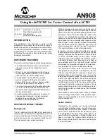
INVERSE PARK
After the PI iteration you have two voltage component
vectors in the rotating d-q axis. You will need to go
through complementary inverse transforms to get back
to the 3-phase motor voltage. First you transform from
the 2-axis rotating d-q frame to the 2-axis stationary
frame
α
-
β
. This transformation uses the Inverse Park
Transform, as illustrated in Figure 4.
FIGURE 4:
INVERSE PARK
INVERSE CLARKE
The next step is to transform from the stationary 2-axis
α
-
β
frame to the stationary 3-axis, 3-phase reference
frame of the stator. Mathematically, this transformation
is accomplished with the Inverse Clark Transform, as
illustrated in Figure 5.
FIGURE 5:
INVERSE CLARKE
Flux Estimator
In an asynchronous squirrel cage induction motor the
mechanical speed of the rotor is slightly less than the
rotating flux field. The difference in angular speed is
called slip and is represented as a fraction of the rotat-
ing flux speed. For example if the rotor speed and the
flux speed are the same the slip is 0 and if the rotor
speed is 0 the slip is 1.
You probably have noticed that the Park and Inverse
Transforms require an input angle
θ
. The variable
θ
represents the angular position of the rotor flux vector.
The correct angular position of the rotor flux vector
must be estimated based on known values and motor
parameters. This estimation uses a motor equivalent
circuit model. The slip required to operate the motor is
accounted for in the flux estimator equations and is
included in the calculated angle.
The flux estimator calculates a new flux position based
on stator currents, the rotor velocity and the rotor elec-
trical time constant. This implementation of the flux
estimation is based on the motor current model and in
particular these three equations:
EQUATION 1:
MAGNETIZING CURRENT
EQUATION 2:
FLUX SPEED
EQUATION 3:
FLUX ANGLE
where:
I
mr
= magnetizing current (as calculated from
measured values)
f
s
= flux speed (as calculated from measured
values)
T = sample (loop) time (parameter in program)
n = rotor speed (measured with the shaft encoder)
T
r
= L
r
/R
r
= Rotor time constant (must be obtained
from the motor manufacturer)
θ
= rotor flux position (output variable from this
module)
ω
b
= electrical nominal flux speed (from motor name
plate)
P
pr
= number of pole pairs (from motor name plate)
During steady state conditions, the I
d
current compo-
nent is responsible for generating the rotor flux. For
transient changes, there is a low-pass filtered relation-
ship between the measured I
d
current component and
the rotor flux. The magnetizing current, I
mr
, is the
component of I
d
that is responsible for producing the
rotor flux. Under steady-state conditions, I
d
is equal to
I
mr
d
and I
mr
. This equation is
dependent upon accurate knowledge of the rotor elec-
trical time constant. Essentially, Equation 1 corrects the
flux producing component of I
d
during transient
changes.
v
α
v
β
Inverse
V
d
V
q
θ
v
α
= V
d
cos
θ
- V
q
sin
θ
v
β
= V
d
sin
θ
+ V
q
cos
θ
β
q
α
v
α
v
β
v
s
θ
V
q
V
d
d
Park
v
α
v
β
v
r1
v
r2
v
r3
β
v
b
v
a
v
c
v
α
v
β
v
s
Inverse
Clarke
v
a
= v
β
v
β
+
√
3 v
α
2
v
b
=
v
β
+
√
3 v
α
2
v
c
=
I
mr
I
mr
T
T
r
-----
I
d
I
mr
–
(
)
+
=
f
s
P
pr
n
⋅
(
)
1
T
r
ω
b
------------
I
q
I
mr
-------
⋅
+
=
θ
θ ω
b
f
s
T
⋅ ⋅
+
=


