


4
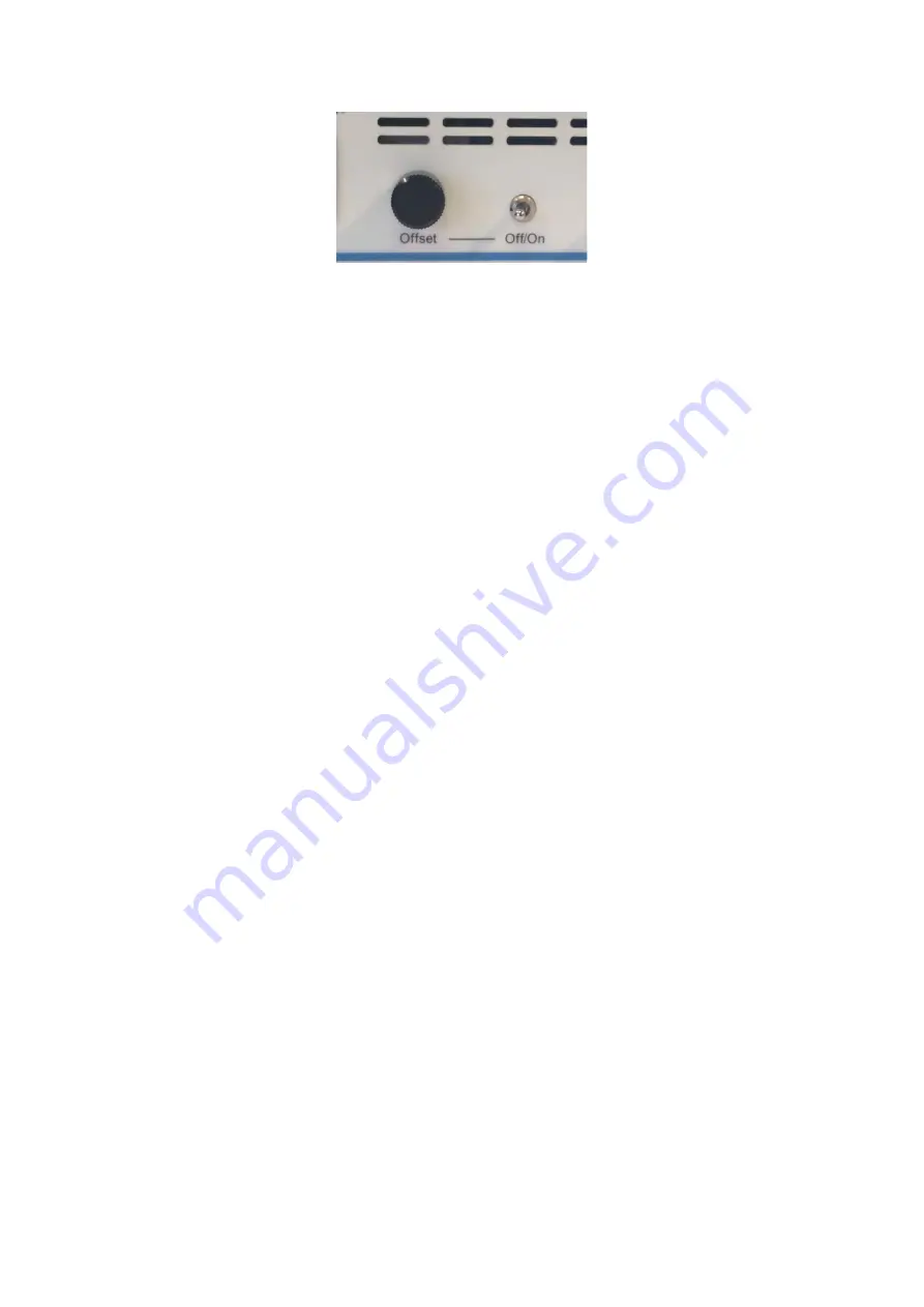
Figure 3. Offset circuitry ‘On-Off’ switch and offset control knob
The load
The output impedance of the WMA-100A
model is 50Ω, to ensure stability with all
capacitive loads. The amplifier is generally
used for high-impedance applications
where the load is capacitive. This is the
case for MEMS devices, EO-modulators
and piezo’s alike. It should be noted that a
coaxial cable itself also presents a
capacitive load of approximately 100pF/m.
The cable that is connected may limit the
maximum
usable
current
at
high
frequencies.
Matched loading with a 50Ω load circuit is
possible by connecting a 50Ω resistor in
series with the output to ground, but is not
recommended. Excessively long cables
will not distort the waveforms, but the
disadvantage is a highly reduced voltage
range (100mA in 50Ω gives 5V maximum
output voltage instead of 170V maximum).
With sensitive and/or high-frequency
measurements, coaxial cables should be
used for connecting both the input and the
output, and their length should be
minimized. If not, the cables will cause
overshoot due to cable reflections (an
effect related to the finite speed of light),
and current limiting due to the cable
capacitance. Although the amplifier itself
remains fully stable, using less than 5
meter of output cable is recommended for
the WMA-100A amplifier to obtain optimal
results.
Transmitter mode
This amplifier can generate a significant
amount of power at frequencies used for
radio transmission and reception. The
amplifier should not be used for
telecommunication as described in the
R&TTE directive 95/5/EC. Always use
coaxial cables.
Amplifier characteristics
In the following pages, several amplifier
characteristics are illustrated:
- Frequency response as a function of
capacitive load (Fig. 4, 5)
- Sine and triangle wave responses (Fig.
6, 7)
- Square wave response (Fig. 8, 9, 10)
- Step response (Fig. 11)
- Capacitive load dependency of square
wave output (Fig. 12)
- Noise with and without offset control
engaged (Fig. 13, 14)
- Rms output noise voltage versus
capacitive load (Fig. 15)