


2-17
IM 701210-05E
Explanation of Functions
2
• Deceleration Prediction
The deceleration curve is computed according to the following equation using the
elapsed time after the pulse input stops (
∆
t).
Frequency (f) = 1/elapsed time (
∆
t)
The deceleration prediction starts after a pulse period (T) of the pulse one period
before the pulse input stopped elapses after the pulse input stopped.
• Stop Prediction
The function determines the stop point at a certain time after the pulse input stops,
and the frequency is set to 0. The time from the point when the pulse input stops to
the point when the function determines that the object has stopped can be set to
×
1.5,
×
2,
×
3, ... ,
×
9, and
×
10 (10 settings) of the pulse period (T) of the pulse one period
before the pulse input stopped.
f
0
T
T
×
n
n: 1.5 to 10
f=1/ t
t
Deceleration prediction
Pulse input stop
Stop prediction
0
Filter
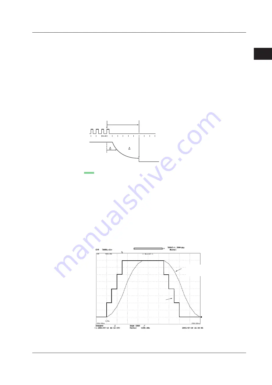
• Smoothing Filter (Moving Average)
The frequency module can display waveforms by taking the moving average of the
data in realtime. The order of moving average can be set in terms of time in the range
of 0.1 ms to 1 s (up to 25000 order). The order of moving average is equal to the
specified time divided by 40
µ
s.
Below are the characteristics of the smoothing filter.
• Converts a waveform that changes in steps to a smooth waveform
• Improves the resolution by reducing the measurement jitter. The resolution
improves when measuring especially high frequencies or when expanding the
display using the offset function. Consequently, highly accurate measurements
can be made.
• Can be used on all measurement parameters of the frequency module.
Original waveform
When using the smoothing filter
Filter order: 400 ms
2.2 Setting the Horizontal and Vertical Axes