Texas Instruments 84PLSECLM1L1T, Руководство пользователя

Страница: 393 / 422

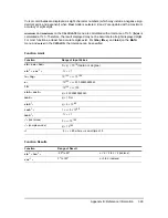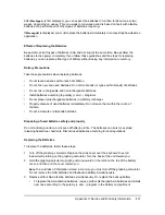
p f
F
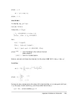
α
∫
x n
1
1 n
2
1 – , – ,
( )
dx =
p f
0
F
∫
x n
1
1 n
2
1 – , – ,
( )
dx =
p
2
--- f x n
1
1 n
2
1 – , – ,
( )
x d
0
L
bnd
∫
f x n
1
1 n
2
1 – , – ,
( )
x d
U
bnd
∞
∫
= =
t
x
1
x
2
–
S
---------------- =
S
Sx
1
2
n
1
-----------
Sx
2
2
n
2
----------- + =
df
Sx
1
2
n
1
-----------
Sx
2
2
n
2
----------- +
⎝ ⎠
⎜ ⎟
⎛ ⎞
2
1
n
1
1 –
--------------
Sx
1
2
n
1
-----------
⎝ ⎠
⎜ ⎟
⎛ ⎞
2
1
n
2
1 –
--------------
Sx
2
2
n
2
-----------
⎝ ⎠
⎜ ⎟
⎛ ⎞
2
+
---------------------------------------------------------------------------- =
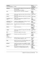
Appendix B: Reference Information 386
2
-
Samp
Ü
Test
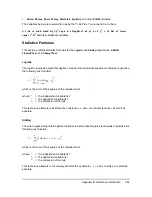
for the alternative hypothesis .
2
-
Samp
Ü
Test
for the alternative hypothesis .
2
-
Samp
Ü
Test
for the alternative hypothesis
s
1
ƒ s
2
. Limits must satisfy the following:
where: [
Lbnd,Ubnd
] = lower and upper limits
The
Ü
-statistic is used as the bound producing the smallest integral. The remaining bound is
selected to achieve the preceding integral’s equality relationship.
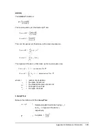
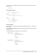
2-SampTTest
The following is the definition for the
2-SampTTest
. The two-sample
t
statistic with degrees of
freedom
df
is:
where the computation of
S
and
df
are dependent on whether the variances are pooled. If the
variances are not pooled:
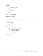
df
(
x, ,
) =
Û
pdf
( ) with degrees of freedom
df
, ,
and
p
= reported
p
value
n
1
1 – n
2
1 – n
1
1 –
n
2
1 –
σ
1
σ
2
>
σ
1
σ
2
<