Teledyne Deltaflow DF180, Operation And Maintenance Manual, Page: 31 / 42

January, 2018
Page 31
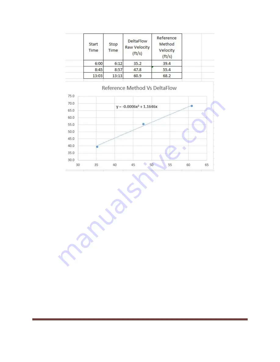
Fig. 5-1 DeltaFlow Correction Curve
Add a linear or up to a 5 th order polynomial trend line. The coefficients of each variable can be entered
into the A0 through A5 fields of the web interface Configuration: Outputs: Computed: Velocity screen
following the form of y = A0 + A1*x + A2*x
2
+ A3*x
3
+ A4*x
4
+ A5*x
5
. For the example in Figure 5-1, A0 =
0, A1 = 1.1646, A2 = -0.0006, and A3, A4, A5 = 0. See section 4.3.3.1.2 for a screenshot of the A0 through
A5 fields. After the coefficients are entered, write the configuration to the controller. Now the Velocity
and Raw Velocity parameters will differ in the Deltaflow as a result of the correction curve. Examining
the graph in Figure 5-1, a Raw Velocity of 40 ft/s would result in a Velocity of 45.
5.4 Long-Term Shutdown
If the Deltaflow is to remain out of service for an extended period of time (greater than 24 hours)
without power, perform the following steps.
1. Disconnect the impact and static pressure lines from the probe.
2. Cap the probe connections with 3/8” tube caps.
3. Perform a blowback sequence to fill the lines with instrument air.
4. Cap the ends of the impact and static pressure lines.
5. Shutoff power to the Deltaflow instrument panel.